Instrumental Variable approach for Causal Inference
If we believe that a variable causes (or affects) another variable , we are often interested in studying how much the value of changes if we make a small change in . For example, how much do people dislike traffic on their street can be measured by decrease in house prices in response to increase in street traffic. The statistical technique most commonly used to answer causal questions is the linear regression [1]
where is the matrix of control variables and we assume that standard OLS assumption holds. However, even when and are causally related, the estimate of is unbiased only if and are independent conditioned on . This is often not the case in practice. In our example, the construction of a new housing development in a neighborhood may increase traffic while lowering the house prices, but this decrease in prices would not be the effect of increased traffic. Similarly, if a shopping complex is built in a neighborhood, it may increase traffic and house prices without this being a causal effect. Instrumental Variable estimation addresses this endogeneity problem by using an instrument that affects only through . By restricting to studying variation in due to variation in that originates through , it is possible to obtain unbiased estimates of .
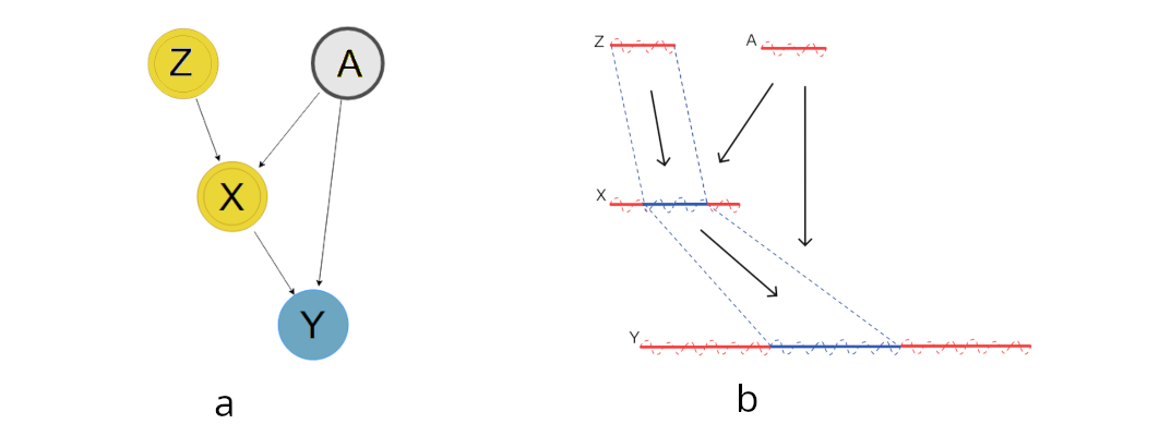
Let us build an intuitive understanding of omitted variable bias in OLS and how IV estimates remove the bias. Consider the causal relation described in figure 1a. is an omitted variable which confounds and . For concreteness, let’s assume that the true data generating process is given by
Assume that and are independent, have mean and variance . The length of line segments in Figure 1b represent the variation in the variables. Without accounting for the omitted variable, the standard OLS gives the incorrect causal estimate
In the IV framework, we use an instrument that affects only through (exogeneity requirement). The IV regression proceeds in 2 stages [2]
In the stage 1, we isolate the variation in caused by the variation in given by . This is represented by the blue part of line segment representing in Figure 1b. This variation is independent of the omitted variable , and we use this variation in to identify the causal effect of on (represented by blue part of ’s line segment). The estimates are given by
which is the correct causal effect of on . Although we only looked at the omitted variable bias, IV method is also useful to correct for “simultaneous causality bias” and the “Errors-in-variables bias”. To wrap our discussions, let us formally state the necessary conditions required for the IV method [3]
- Relevance: The instrument variable should be correlated with the causal variable of interest . This can be easily checked from significance level of the first stage estimate. Higher correlation in the first stage means that the instrument can more effectively extract the exogenous variation in the regressor and hence the causal estimate has a lower standard error.
- Exogeneity: The instrument variable is uncorrelated with the error term in the regression equation ( where is a vector of controls). Since the error term in unobserved, this condition is not statistically testable and needs to be justified theoretically. Sometimes, this is specified as the combination of exclusion restriction and as-if random condition.
- Exclusion Restriction: Fixing controls , the instrument affects outcome only through .
- As-if random: Fixing controls , the instrument itself must not be endogenous. This rules out any reverse causality from to .
Shift-Share instruments
In many economic settings, the shocks that a researcher would like to use as instruments operate at a different level than the units being studied. For example, a researcher studying regional labor markets may find plausibly exogenous variation at the industry level — such as changes in trade policy, technology, or national demand that hit specific industries. But the outcome equation is specified at the regional level, because that is where workers live, earn wages, and make decisions.
The shock does not map one-to-one onto regions: a single industry shock affects many regions, and a single region is exposed to many industry shocks, each to a different degree depending on its industrial composition. Shift-share instrumental variables (also known as Bartik instruments) provide a principled way to translate these shock-level instruments to the unit level. This section draws on the practical guide by Borusyak, Hull, and Jaravel (2025).
Structure of a shift-share instrument
Consider a model where we wish to estimate the causal effect of treatment on outcome across units :
where is a vector of controls. As before, OLS is biased when is correlated with . Suppose that a set of shocks at some other level (industries, origin countries, age groups, etc.) are plausibly exogenous. Each unit has a known vector of exposure shares that capture how much unit is exposed to each shock . The shift-share instrument aggregates these into a single unit-level variable:
When the shares sum to one, is a share-weighted average of the shifts. The instrument inherits its exogeneity from the shifts, while the shares give it cross-sectional variation at the unit level — different regions are affected differently by the same set of national shocks because their industrial compositions differ.
Example 1: Inverse elasticity of regional labor supply
The canonical example is Bartik’s (1991) instrument for local labor demand. Suppose we want to estimate the inverse elasticity of regional labor supply by relating wage growth to employment growth across regions . Local employment can be decomposed across industries:
where is the initial employment share of industry in region , and is the local industry growth rate. To isolate demand-driven variation, the Bartik instrument replaces local industry shifts with national industry growth rates , while keeping the local shares . The national growth rates proxy for aggregate demand shifts and should be uncorrelated with local labor supply shocks.
Example 2: US labor market impact of Chinese import competition
Autor, Dorn, and Hanson (2013) study how Chinese import competition affected US local labor markets. Their treatment is the change in import exposure per worker in commuting zone , measured as a share-weighted sum of industry-level changes in US imports from China. Since realized US imports may reflect US-specific demand shocks, they instrument with Chinese import growth in eight other high-income countries:
where is region ’s lagged share of national employment in industry , and is the change in imports from China to other developed markets in industry . Lagged employment avoids simultaneity. The identification relies on China’s export surge being driven by internal supply-side factors (productivity growth, WTO accession) rather than correlated demand shocks across importing countries.
Two paths to identification
As discussed above, the causal identification in the IV method requires the instrument to be relevant and exogenous. The core challenge with any shift-share instrument is arguing that is exogenous, i.e. uncorrelated with . Since combines two distinct sources of variation — shifts and shares — there are two paths to making this argument.
Path 1: Exogenous shifts
The first strategy places the exogeneity burden on the shifts. If each shift is as-good-as-randomly assigned and only affects the outcome through the treatment, then a weighted average of many such random shifts will also be exogenous. The intuition is that of a “weighted average of lotteries”: if each industry shock is like an independent draw, then the shift-share instrument — which averages across many of them — inherits this randomness by a law of large numbers argument.
What makes this powerful is that the shares need not be exogenous at all. Regions that specialize in high-skill industries may have systematically different unobservables from those that specialize in low-skill industries. But as long as the shocks hitting high-skill and low-skill industries are themselves random, these compositional differences wash out in expectation.
More formally, exogeneity of the instrument requires a weaker condition than full randomization of each :
This is sufficient for . In words: each shift shock must not be systematically correlated with the idiosyncratic unobservables of the units most heavily exposed to it.
Returning to the China shock example: even if regions with more manufacturing employment have systematically different labor market trends, the instrument is valid as long as China’s productivity shocks across industries are unrelated to US regional labor market conditions.
Requirements:
- Many shifts are necessary. Otherwise, there might be spurious correlation between shift shocks and average idiosyncratic shocks .
- Shares must sum to one for each unit (). Otherwise, if shares do not sum to one, then where . Units with a larger sum of shares systematically get higher values of the instrument, and this sum may be correlated with , creating bias. Including as a control resolves this.
Practical considerations:
- Shift-share aggregates of any shift-level confounders should be included as controls (i.e. control for )
- Shares should be lagged to the beginning of the natural experiment to avoid the shifts themselves reshaping the shares
- Standard errors should be “exposure-robust”, obtained from the equivalent shift-level IV regression (available via the
ssaggregatepackage in Stata and R)
Path 2: Exogenous shares
A different strategy assumes that the exposure shares are exogenous. This can be interpreted as each share satisfying a parallel trends condition: outcomes of units with high versus low values of would have trended similarly absent the treatment .
Under share exogeneity, the shift-share estimate can be viewed as pooling together “one-at-a-time” estimates, each using a single share as the instrument. The exogenous shares approach is appropriate when the researcher is comfortable using any of the individual shares as an exogenous instrument — that is, when there are no conceivable unobserved shocks that affect the outcome via the same shares used to construct the instrument. This is bolstered when the shares are “tailored” to the treatment, in the sense of mediating only the shocks to and not a broad set of shocks that might affect .
For example, Card (2009) studies the effect of immigration on native wages across US cities. The share is the fraction of immigrants from origin country living in city in 1980, and the shift is the national inflow of immigrants from country in later decades. The share of Cuban immigrants in Miami, say, is a plausible instrument because it is “tailored” — it captures exposure specifically to Cuban immigration shocks, not to labor market shocks in general. The parallel trends assumption is that cities with high versus low Cuban immigrant shares would have seen similar wage trends absent the immigration surge.
Practical considerations:
- Shares must be “tailored” to the treatment, not “generic” (capturing exposure to many types of shocks)
- Balance tests should be performed on individual shares, focusing on those with high Rotemberg weights
- Rotemberg weights (computed via the
bartik_weightcommand) measure the importance of each share instrument and the sensitivity of the estimate to violations of exogeneity for each share - Sensitivity to alternative ways of combining share instruments should be checked (e.g. overidentification tests, visual instrument variable plots)
- Standard heteroskedasticity- or cluster-robust standard errors are appropriate
Choosing between the two approaches
| Exogenous Shifts | Exogenous Shares | |
|---|---|---|
| Identification | Shifts are as-good-as-randomly assigned and only affect outcome through treatment | Each share satisfies parallel trends: units with high vs. low shares would have trended similarly absent treatment |
| Estimation | Control for sum of shares (if not one) and shift-share aggregates of shift-level controls | Check robustness to using share instruments directly (e.g. one share at a time, or pooled via 2SLS/LIML/GMM) |
| Inference | Exposure-robust standard errors from equivalent shift-level IV regression | Conventional heteroskedasticity- or cluster-robust standard errors |
| Balance tests | For both the shift-share instrument and the shifts | For both the instrument and shares with high Rotemberg weights |
| Do not use when… | Shifts are too few or endogenous to use directly as instruments | Shares are “generic” (capturing exposure to many types of shocks) |
In some settings one approach is clearly more appropriate. For instance, the exogenous shifts approach requires many shifts for the law of large numbers argument to work, while the exogenous shares approach requires shares that are tailored to the specific treatment. In other settings, thinking through the potential bias and efficiency properties under each approach can help the researcher decide.
References
- Autor, David H., David Dorn, and Gordon H. Hanson. 2013. “The China Syndrome: Local Labor Market Impacts of Import Competition in the United States.” American Economic Review 103(6): 2121–68.
- Bartik, Timothy J. 1991. Who Benefits from State and Local Economic Development Policies? W. E. Upjohn Institute for Employment Research.
- Borusyak, Kirill, Peter Hull, and Xavier Jaravel. 2022. “Quasi-Experimental Shift-Share Research Designs.” Review of Economic Studies 89(1): 181–213.
- Borusyak, Kirill, Peter Hull, and Xavier Jaravel. 2025. “A Practical Guide to Shift-Share Instruments.” Journal of Economic Perspectives 39(1): 181–204.
- Card, David. 2009. “Immigration and Inequality.” American Economic Review 99(2): 1–21.
- Goldsmith-Pinkham, Paul, Isaac Sorkin, and Henry Swift. 2020. “Bartik Instruments: What, When, Why, and How.” American Economic Review 110(8): 2586–2624.
- Adão, Rodrigo, Michal Kolesár, and Eduardo Morales. 2019. “Shift-Share Designs: Theory and Inference.” Quarterly Journal of Economics 134(4): 1949–2010.